Geomodeling Guides Jonah Infill Wells
The Jonah Field in the Green River Basin in Sublette County, Wyoming is one of the most prolific natural gas fields in the Rocky Mountain region, estimated to contain up to 15 trillion cubic feet of natural gas in a 32 square mile productive area. The field is defined by the intersection of two sub-vertical shear fault zones that form a wedge-shaped structural block. To evaluate infill well development in various sections of the Jonah Field, reservoir characterization and simulation studies were performed to integrate geology, Petrophysics, 3-D seismic and engineering data into technically sound 3-D geologic and engineering models. The reservoir characterization and simulation work focused on three sections within the main field area. Detailed geomodels were built for each section, from which reservoir simulation models were then extracted. The studies included: Detailed Petrophysical modeling for minerals, effective porosity and fluid saturations; Well-and seismic-based interpretations of internal markers within the Lance formation; Calibrating with cores and thin section images; Generating log-based vertical facies proportion curves; Generating a facies probability cube based on log facies and seismic information; and constructing an integrated 3-D geomodel.
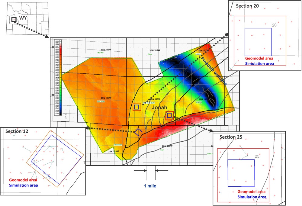
Figure 1 : Jonah Field: location and study areas
Figure 1 shows the locations of the three study areas at Jonah Field. Most of the production comes from overpressured and ultra tight Lance Sandstones.
Facies Characterization
Characterizing the facies geometry focused on identifying pay and nonpay facies using core and well log data. Pay facies consist of single and multistory channels. Facies geometry was characterized using three methods to capture different scales and variability across each area:
- Local facies curves to capture the local facies variability at each well location;
- Vertical proportion curves to capture the global vertical facies variability for a whole area (a section, for instance); and
- Seismic-driven facies probability cubes to capture the spatial variations in facies distributions and to use as “soft constraint” when integrating all the facies information into a single geomodel (local facies curves and vertical proportion curves were treated as hard data when building the geomodel).
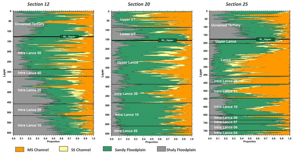
Figure 2 : Facies proportion curves
Stratigraphic Correlations
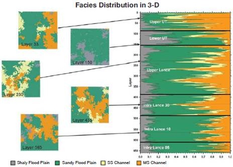
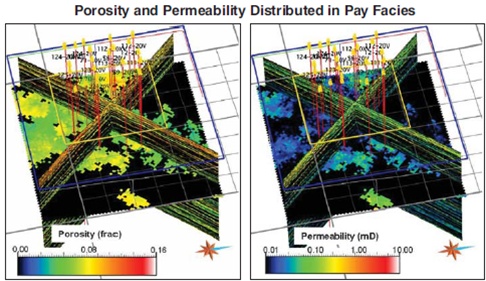
Stratigraphic correlations were performed using lithology and facies logs. After several iterations between stratigraphic correlations among different wells and careful seismic interpretation (usually performed in a line-by-line fashion), a set of seismic horizons and well markers were obtained that were totally consistent with one another. The seismic horizons were also used as a guide to pick additional well markers that were not visible in the log data. Figure 2 shows the “facies proportion curves” and are used to estimate and constrain the relative amounts of each facie in each layer of the geomodel. From left to right, the plot for each section shows the relative proportion of shaly flood plains, sandy flood plains, single-story channels, and multistory channels, respectively. Facies information derived from well and seismic data was used to constrain the facies distribution in the geomodel. Figure 3 shows the result of the 3-D facies distribution in selected layers of the model for one of the study areas. The image at right is the vertical proportion curve, while the diagrams at left are areal slices for particular stratigraphic slices. Figure 4 shows the result of the porosity and permeabilitymodeling. Porosity and permeability in nonpay facies was set to zero (black coloring).
|
|
|
Figure 3 : Facies distribution in 3D |
Figure 4 : Porosity and permeability distributed in pay facies |
Multiwell Simulation
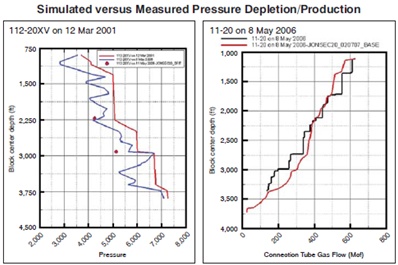
Figure 5 : Simulated versus measured pressure depletion/production
The multiwell simulation performed for this project attempted to address longterm well performance, including well interference effects and optimal spacing. Only minimal upscaling of the geologic model was undertaken for simulation in order to preserve the complex architectural elements. In this case, it was important to maintain detailed geologic descriptions throughout the model area rather that using coarse grids with nearwell refinements, as is commonly applied. Laboratory-measured compaction data was used to account for permeability loss as pore pressure was reduced. This has important implications on long-term recovery. For pressure initialization, separate pressure regions were assigned according the defined stratigraphic intervals, with initial pressures determined from the regional overpressure gradient (1.16 psi/foot). The models were validated by matching tubing-head pressures while honoring historical gas rates.
Figure 5 shows that the simulated depletion data at a recent infill well (blue versus red line) is similar in magnitude to the measured pressure depletion (symbols). Measured production inflow (the black line on the figure at right) also was approximated by the simulator (red line).
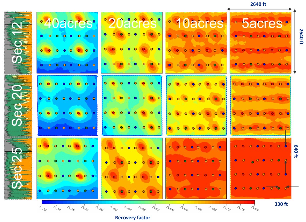
Figure 6 : Simulated long-term recovery maps
Predicting Well Performance
After validating the model, forecasts were performed in which the simulator estimated future gas rates using tubinghead or bottom-hole pressure constraints. Figure 6 shows comparisons of long-term recovery for uniform well spacing. Well spacing is elongated to allow for elliptical drainage in northwest-to-southeast direction based on maximum stress and depositional geometry.
The left column shows the Jonah section number on top of the facies proportion curve, with well spacing varying from 40 to five acres moving from left to right. Blue represents 20 percent recovery of original gas in place, while red represents 80 percent recovery. The Lance interval shows large variations in the proportion of pay intervals across the field, as illustrated by the detailed reservoir characterization of the three separate areas described in this article. These variations will have a considerable impact in the development plans and economic forecasts. Successful reservoir characterization of this kind of geologically complex reservoir depends to a large extent on how all the diverse information is applied in a way that is both consistent and complementary. Details are important and numerous iterations between disciplines may be required to ensure data consistency.
For more information: “Infill well evaluations of Jonah Field tight gas: characterization and simulation of complex architectural elements”, Reinaldo J. Michelena, James R. Gilman, Omar Angola, Mike J. Uland and Ira Pasternack, First Break, volume 27, April 2009.